Root Mean Square Velocity Calculator

Random RMS Figurer Tutorial

Calculators and Tools

Compute random dispatch, velocity, and displacement values from a breakpoint table.

Complete RMS Estimator (Excel)

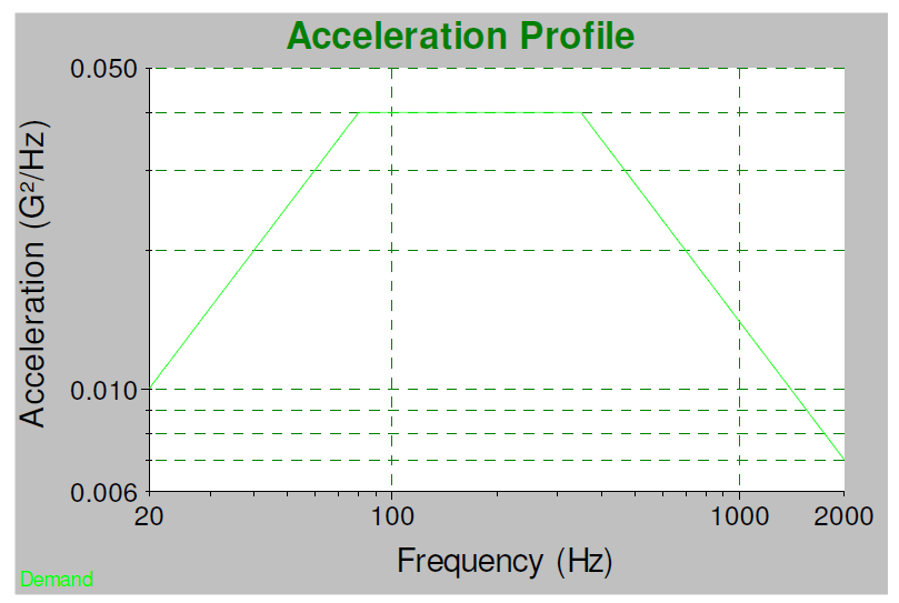
A random spectrum is defined every bit a set up of frequency and aamplitude breakpoints. Consider the values on the tabular array below:

Frequency (Hz)	Amplitude
20	0.01005
80	0.04000
350	0.04000
2000	0.00704

random-rms

To compute the root hateful square (RMS) from the breakpoint values, we must calculate the area under the curve defined past the breakpoint values. At first, this may seem elementary because it tin be divided into a group of squares and triangles. However, the triangles are the result of straight lines on log-log graph paper, not linear. Nosotros can yet take advantage of the triangle shapes but need to employ a specific formula to compute the area of triangles on log-log graph paper.

The definition of a straight line on log-log graphs between ii breakpoints (f1,a1) and (f2,a2) is a power relationship, where the slope is the exponent, and the outset is the multiplicative factor.

(1) $\begin{equation} a=\text{offset}\times f^{slope} \end{equation}$	(i)

The slope and offset that define the direct line are computed as follows:

(2) $\begin{equation} \text{slope}=\frac{\log(a_{2})-\log(a_{1})}{\log(f_{2})-\log(f_{1})} \end{equation}$	(2)

(3) $\begin{equation} \frac{a_{1}}{f_{1}^{slope}} \end{equation}$	(iii)

Given the slope and offset, we tin integrate from f₁ to f₂ to compute the area under the line:

(four) $\begin{equation} \text{area}=\left[\frac{\text{offset}}{(\text{slope}+1)}\right]\times[f_{2}^{(slope+1)}-f_{1}^{(slope+1)}]\text{, if slope}\neq1 \end{equation}$	(4)

However, this formula does not concord if the slope equals 1. In this instance, we note that a = showtime / f, which integrates into a natural log role.

Hint: some programs such equally Microsoft Excel^TM define the log() function as a base-x logarithm and the ln() function as the natural (base-e) logarithm. Exist sure to use the correct role in your calculation. Equally a examination, log(ii.71828182845905) = 1.0 for a natural logarithm.

(five) $\begin{equation*} \text{area}=\text{offset}\times(\ln(f_{2})-\ln(f_{1}))\text{, if slope}=-1 \end{equation*}$

(5)

Nosotros tin can apply Equations (4) or (5) to calculate the area under the curve for each pair of breakpoints. The total area is the sum of the individual area calculations between each breakpoint pair and is the mean-square acceleration. The square root of the upshot equates to the RMS acceleration level. If nosotros use the example breakpoints, the sum is computed as follows:

Frequency (Hz)	Amplitude (G²/Hz)	Slope	Start	Expanse (G²)
20	0.01005
fourscore	0.04000	0.9964	0.000508	1.fifty
350	0.04000	0	0.04000	ten.eighty
2000	0.00704	-0.9967	13.73	24.47
				Total 36.77 Gⁱⁱ

(6) $\begin{equation*} \sqrt{36.77\text{ G}^{2}} = 6.064\text{ G} \end{equation*}$

The sum of the area values equates to a mean-square acceleration of 36.77 G^two. The square root of this value gives an overall RMS value of half dozen.064 One thousand RMS. The dispatch units are the foursquare root of the acceleration density units. For a density unit of (chiliad/due south²)²/Hz, the upshot will have a unit of 1000/s². For a density unit of measurement of 1000^two/southward³ (a reduced form of (m/s²)ⁱⁱ/Hz), the upshot will have a unit of yard/southward².

WHAT About VELOCITY?

The RMS velocity can be computed the aforementioned equally acceleration; however, the breakpoint values must be converted from units of acceleration-squared/Hz to velocity-squared/Hz with appropriate unit conversion if required. This conversion is performed with Equation (half dozen), which defines the relationship betwixt velocity and acceleration for a sine wave of a given frequency.

(7) $\begin{equation} \text{velocity}=\frac{\text{acceleration}}{2\Pi f} \end{equation}$	(6)

As a result, the equation in velocity density for the lines connecting the breakpoints becomes:

(8) $\begin{equation} \frac{\text{offset}}{(2\Pi)^{2}}\times f^{(slope-2)} \end{equation}$	(7)

This tin be integrated from f_ane to f₂ to equate the area under the velocity line.

(9) $\begin{equation} \frac{1}{(2\Pi)^{2}} \frac{\text{offset}}{(\text{slope}-1)} ({f_{2}^{slope-1}) - ({f_{1}^{slope-1})\text{, slope}\neq 1 \end{equation}$	(8)

When slope = ane, nosotros must use a natural log function.

(ten) $\begin{equation} \text{area}=\frac{\text{offset}}{(2\Pi)^2}\times(\log(f_{2})-\log(f_{1}))\text{, slope}=1 \end{equation}$	(9)

Then, we tin sum the areas to calculate the mean-square velocity, and take the square root of the value to get RMS velocity for the random spectrum. When using acceleration unit of measurement G, we must also apply a conversion cistron to get a suitable velocity unit of measurement. Common conversions are K to inches/s² or thou/south².

(11) $\begin{equation} 1\text{G}=386.09\text{in/s}^2=9.80665\text{m/s}^2 \end{equation}$	(10)

Using the previous example, the RMS velocity is computed equally follows:

Frequency (Hz)	Aamplitude (Chiliad²/Hz)	Slope	Starting time	Area ((G $\cdot$ s)²)
20	0.01005
80	0.04000	0.9964	0.000508	1.760e-5
350	0.04000	0	0.04000	0.977e-five
2000	0.00704	-0.9967	13.73	0.141e-v
				Full 2.878e-v

(12) $\begin{equation*} \sqrt{2.878e-5(\text{G}\times\text{s})^2} = 0.005364\text{G}\times\text{sRMS} \end{equation*}$

Applying the unit conversion, we get:

(13) $\begin{equation*} 0.005364\text{G}\times\text{s}\times\frac{386.09\text{in/s}^2}{1\text{G}}=2.07\text{in/s RMS} \end{equation*}$

WHAT Well-nigh Displacement?

The RMS displacement tin can too be computed the same as acceleration; however, the breakpoint numbers must be converted from units of dispatch-squared/Hz to displacement-squared/Hz with advisable unit conversion if required. This conversion is performed with Equation (11), which defines the relationship between acceleration and displacement for a sine wave of a given frequency.

(14) $\begin{equation} \text{displacement}=\frac{\text{acceleration}}{(2\Pi f)^2} \end{equation}$	(11)

Every bit a event, the equation for the lines connecting the breakpoints in displacement density becomes:

(15) $\begin{equation} d=\frac{\text{offset}}{(2\Pi)^4}\times f^{slope-4} \end{equation}$	(12)

At present, we can integrate this from f_one to f_ii to get the area under the displacement line.

(xvi) $\begin{equation} area=\frac{1}{(2\Pi)^4}\frac{\text{offset}}{\text{slope}-3}(f_{2}^{slope-3}-f_{1}^{slope-3})\text{ slope}\neq3 \end{equation}$	(13)

When gradient = iii, nosotros need to use a natural log part:

(17) $\begin{equation} area=\frac{\text{offset}}{(2\Pi)^4}\times(\log(f_{2})-\log(f_{1}))\text{ slope}=3 \end{equation}$	(14)

Then, we can sum the areas to become the mean-foursquare deportation and take the foursquare root of the value to become RMS displacement for the random spectrum. When using acceleration units in M, y'all also need to utilize a conversion gene such as Equation (ten) to get a suitable displacement unit.

Using the previous example, the RMS displacement is computed as follows:

Frequency (Hz)	Amplitude (G^two/Hz)	Slope	Offset	Area ((One thousand $\cdot$ sⁱⁱ)²)
20	0.01005
80	0.04000	0.9964	0.000508	three.773e-10
350	0.04000	0	0.04000	0.165e-10
2000	0.00704	-0.9967	thirteen.73	0.0015e-10
				Total 3.994e-10

(18) $\begin{equation*} \sqrt{3.994e-10(G\times s^{2})^{2}}} = 1.985e-5 G\times s^{2} RMS \end{equation*}$

After applying the unit conversion, we become:

(19) $\begin{equation*} 1.985e-5 G\times s^{2}\times\frac{386.09in/s^{2}}{1G}=0.0077\text{ in RMS} \end{equation*}$

Notwithstanding, nosotros are more likely to exist interested in peak-to-peak displacement rather than RMS displacement considering shaker travel limits are rated every bit a peak-to-height value. The vibration is Gaussian random, then information technology is not possible to find an accented peak value. Nevertheless, we can compute an average or typical summit value. For Gaussian random values, the average one-sided peak level is almost iii times the RMS value (also called the three-sigma level). To go double-sided displacement—eastward.g., peak-to-peak deportation—this number is doubled.

The typical peak-to-peak value is computed as:

Typical elevation-pinnacle displacement = 2 · 3 · (0.0077 in RMS) = 0.046 in peak-to-summit

Information technology is important to understand that this value is the typical peak-to-top displacement value and will occur relatively ofttimes during the test. Yet, you will also take occasional peaks at levels higher than three·RMS. These peak heights can just exist defined in terms of probabilities. Therefore, the appropriate question is not how high the peaks are but how often they will reach that height.

For Gaussian random information, the amplitudes will exceed 3·RMS 0.27% of the fourth dimension and iv·RMS 0.006% of the time. There is a 0.0000002% take a chance that a peak volition exceed 6·RMS. This probability is small but not impossible. In practice, 30% to fifty% of the headroom should exist above the typical peak-to-peak displacement value to account for the occasional higher peak levels.

WHAT ABOUT SINE-ON-RANDOM?

Sine-on-Random tests have groundwork random vibration with one or more than sine tones overtop. The groundwork random levels are computed the aforementioned as standard random as described to a higher place. The sine tones add to the random in the mean-square. We must sum all the squared values of the RMS levels, then take the foursquare root of the issue to calculate the overall RMS value. The sine tones are unremarkably divers by their peak acceleration, and so they must be converted from superlative to RMS. For a sine tone, this is equally unproblematic every bit dividing the acme value by the square root of 2.

Sine-on-Random Example

Using the background random as defined above and add together sine tones of one.0G elevation at 50Hz, two.0G peak at 80Hz, and 1.5G superlative at 110Hz.

Frequency (Hz)	Acceleration One thousand Peak	Acceleration Grand RMS	Squared One thousandⁱⁱ
Random	–	half-dozen.064	36.77
50	ane.0	0.707	0.fifty
80	2.0	one.414	2.00
110	i.five	i.061	i.thirteen
			Total forty.twoscore

(20) $\begin{equation*} \sqrt{40.40G^{2}}=6.36G\text{ RMS} \end{equation*}$

Velocity functions the same style. Convert the acceleration to velocity using Equation (six), then catechumen the result to the advisable velocity unit of measurement. When summing the squared values, the units for the groundwork random and the sine tones should match.

(21) $\begin{equation*} \sqrt{4.411e-5(G\times s)^{2}} = 0.006642 G\times s RMS \end{equation*}$

Applying the unit conversion, nosotros get:

(22) $\begin{equation*} 0.006642 G\times s\times\frac{386.09 in/s^{2}}{1G} = 2.56 in/s RMS \end{equation*}$

Displacement would function the same fashion if we were interested in RMS values. All the same, to go peak deportation, the peak-to-peak sine displacement would exist ii times the square root of 2 multiplied by the RMS displacement for the sine tones. The RMS-to-(peak-to-height) conversion gene for 3-sigma random peaks (equally assumed for the random groundwork vibration) would not use to the sine tones.

To run into the overall superlative-to-peak displacement requirements, it is better to presume that the peaks for the sine tones and the random groundwork could occur at the aforementioned indicate in time. As such, the top displacement values are simply added together.

To go the overall sine-on-random peak-to-top displacement requirement, add together the peak-to-tiptop displacements for the random background and each of the sine tones. Convert acceleration to displacement using Equation (11), then catechumen the displacement units using Equation (10).

Frequency (Hz)	Dispatch (G Pk)	Displacement (G $\cdot$ s^two pk-pk)	Displacement in pk-pk
random	–	–	0.046
50	i.0	1.433e-5	0.006
80	2.0	0.112e-5	0.004
110	1.5	0.444e-v	0.002
			Total 0.058 intiptop-to-peak

Consummate RMS Figurer (Excel)